Introduction to Parameter Estimation
Why Parameter Estimation is Important
Parameter estimation constitutes a foundational component of modeling and simulating real-world systems, batteries included. It entails the process of utilizing measurement data to determine the values of parameters within a mathematical model that mirrors a physical system. In battery modeling, these parameters may encompass internal resistance, diffusion coefficients, reaction rates, and various other physical properties. The significance of parameter estimation in battery modeling derives from several key aspects:
Accuracy: Precise parameter values are of paramount importance to ensure that the model closely mirrors the actual behavior of the battery. This level of accuracy proves critical in predicting battery performance, safety, and lifespan.
Adaptation to Variability: Due to disparities in manufacturing, the effects of aging, and fluctuations in operating conditions, batteries can exhibit variability. Parameter estimation serves as a means to enable models to adapt to this variability, guaranteeing that predictions remain relevant and precise.
Optimization and Control: In applications like Battery Management Systems (BMS), the acquisition of accurate parameters is imperative. These parameters form the basis for optimizing charging and discharging strategies and are instrumental in ensuring the secure operation of batteries.
Design Decisions: Engineering decisions about the design and selection of batteries for particular applications are based on realistic models. The precision of the model parameters determines how reliable these decisions are.
Common Techniques in Parameter Estimation
Least Squares Estimation: One of the most popular methods is called least squares estimation, and it entails minimizing the sum of the squares of the discrepancies between the values that were observed and those that were predicted by the model. Dealing with noisy data calls for the use of this technique particularly well.
Maximum Likelihood Estimation (MLE): Maximum Likelihood Estimation (MLE) stands as a method employed to determine parameters in a model by identifying the values that maximize the likelihood of the observed data under the given model. This approach proves particularly valuable when there exists a known probability distribution that characterizes the process of data generation.
Bayesian Estimation: In contrast to Maximum Likelihood Estimation (MLE), Bayesian Estimation integrates prior knowledge or beliefs regarding the parameters by representing them as a probability distribution. These beliefs are then updated with new data to derive parameter estimates.
Gradient-Based Optimization: Algorithms like Gradient Descent are employed in Gradient-Based Optimization. These algorithms iteratively modify the parameters in a manner that diminishes the disparity between model predictions and observed data.
Genetic Algorithms: Inspired by natural selection and genetics, genetic algorithms serve as optimization algorithms. They are adept at approximating solutions to optimization and search problems and can be harnessed for parameter estimation.
System Identification: This is a method especially relevant in control engineering. It involves the determination of the model structure and the fine-tuning of parameters based on input-output data.
Parameter estimation proves to be an iterative and often computationally demanding process. The selection of suitable methods hinges on factors such as the model's nature, the available data, and the specific demands of the application. Moreover, the quality of the parameter estimates should undergo validation through techniques like goodness-of-fit metrics and cross-validation.
Parameter Estimation for Electrochemical Models
Fitting Techniques
In the domain of electrochemical models, precise parameter estimation plays a pivotal role in ensuring an accurate depiction of the physical and chemical phenomena unfolding within batteries. These parameters encompass aspects such as reaction kinetics, solid-phase, and electrolyte diffusion coefficients, and exchange current densities, among others. To derive estimates for these parameters, a range of fitting techniques can be employed.
Curve Fitting: This method entails the fitting of a curve or mathematical function to a collection of experimental data points. In the context of electrochemical models, this might involve the fitting of voltage curves or concentration profiles to empirical data. Various curve-fitting techniques can be applied for this purpose. The following list, while not exhaustive, provides an overview:
- Linear fitting, with respect to the square-root of the step time
- Exponential fitting, where an exponential is fit to the experimental data
- Perform direct-pulse fitting by directly matching the voltage to a one-dimensional electrochemical model. This approach aims to replicate the same characteristics and calculate the diffusion coefficient.
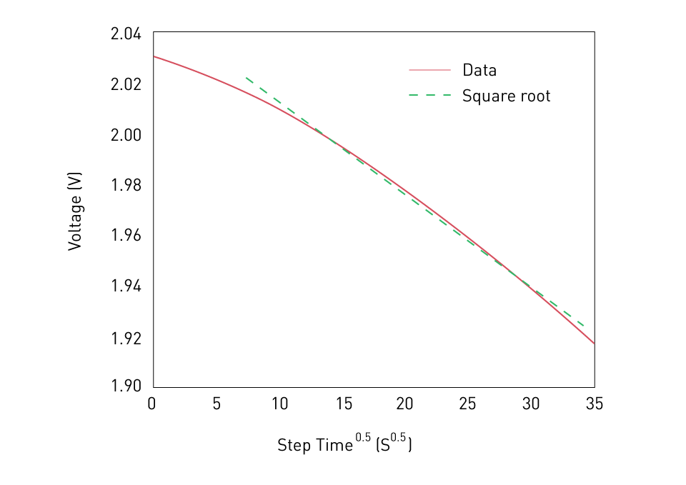
Figure 10: Linear fitting method
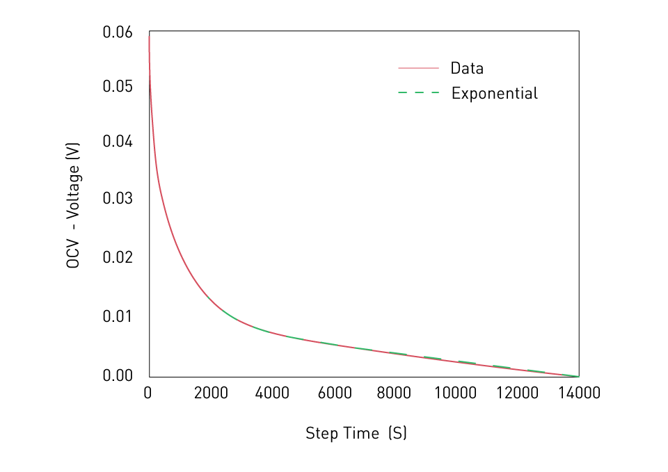
Figure 11: Exponential fitting

Figure 12: Direct-pulse fitting
Optimization Algorithms: Given the nonlinearity inherent in electrochemical models, optimization algorithms such as simulated annealing or genetic algorithms frequently come into play. These algorithms are employed to minimize the disparity between model predictions and empirical data. The objective is to identify a parameter set that results in the least deviation between the model and the actual data.
Parameter Sweeping: This approach entails a systematic alteration of one or more parameters across a predefined range, observing the resultant impact on the model's output. It becomes possible to refine the range of plausible values for the parameters by comparing this output with empirical data.
Parameter Sensitivity Analysis
Parameter Sensitivity Analysis constitutes a systematic technique for examining how the uncertainty associated with the output of an electrochemical model can be attributed to distinct sources of uncertainty in its parameters. It basically quantifies how variations in input parameters influence the model's output. In the realm of electrochemical modeling, this holds significance for several reasons:
Identifying Key Parameters: Sensitivity analysis aids in determining which parameters have a substantial impact on the output of the model. This makes it possible to prioritize the parameters that require more precise estimation.
Refining Model Complexity: It is possible to decide whether a model may be simplified, which can be especially helpful in easing the computing burden by analyzing the sensitivity of model outputs to various factors.
Robustness and Uncertainty Quantification: Determining the robustness of model predictions and quantifying prediction uncertainty require an understanding of how sensitive a model is to changes in parameters.
Methods for conducting sensitivity analysis include:
Local Sensitivity Analysis: This method revolves around computing the derivative of the model's output concerning each parameter. In essence, it quantifies how a minor alteration in a parameter influences the model's output.
Global Sensitivity Analysis: Unlike local techniques, global sensitivity analysis takes into account the complete parameter space. Approaches like the Sobol’ indices assess the contribution of each parameter to the output variance over its entire range.
Monte Carlo Analysis: This technique entails running the model multiple times, with parameters drawn from probability distributions that depict their uncertainty. Subsequently, the resulting distribution of outputs is analyzed.
Parameter Estimation for ECMs
Equivalent Circuit Modeling stands as the most predominant approach for the analysis of batteries. As we've already established, the parameters of primary interest within this context encompass the series and parallel resistances, along with the parallel capacitors featured in the model.
Least Squares Methods
They emerge as a widely employed technique when it comes to estimating parameters for Equivalent Circuit Models (ECMs). This method involves the fitting of a curve onto a series of measurement data points (depicted in red), with the objective of minimizing the sum of the squares of the differences between the measured data and the estimated curve (illustrated in blue). In the realm of battery ECM models, the method culminates when it successfully identifies the resistance and capacitance components of the circuit that yield the minimal sum of squares.
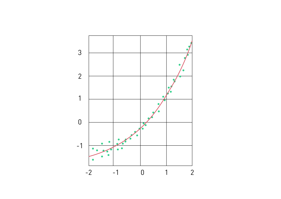
Figure 13: Least Square Method
Linear Least Squares: In scenarios where the ECM takes on a linear form, linear least squares prove to be an applicable method. This approach entails the identification of a line (or hyperplane) that minimizes the sum of squared residuals, which are essentially the vertical distances between the data points of the dataset and the fitted line.
Nonlinear Least Squares: For ECMs that exhibit nonlinear characteristics, the Nonlinear Least Squares method is better suited. This technique generalizes the linear least squares approach to accommodate nonlinear models. It iteratively modifies the parameters to minimize the sum of squared residuals.
Both linear and nonlinear least squares problems can be solved using software tools such as MATLAB and Python libraries.
System Identification
This is an approach utilized to construct mathematical models of dynamic systems by observing the system's response when it is stimulated with specific signals. In the context of ECMs, system identification methods can be harnessed to deduce the values of various electrical components (such as resistors and capacitors) that most accurately represent the battery's behavior.
Frequency Response Analysis: The system's frequency response can be ascertained by exposing it to sinusoidal excitation signals of varied frequencies and examining the response. The electrical components in the ECM's electrical components can be estimated using this information. The Nyquist diagram is used to show the excitation's outcomes. A point on the diagram is represented by every excitation frequency. The complex impedance of the battery can be seen in the diagram varying with frequency. Going from left to right, zones of high frequency and low frequency can be distinguished. Each zone represents a separate phenomenon in the battery, such as diffusion (low frequency) and charge-transfer reaction (high frequency).
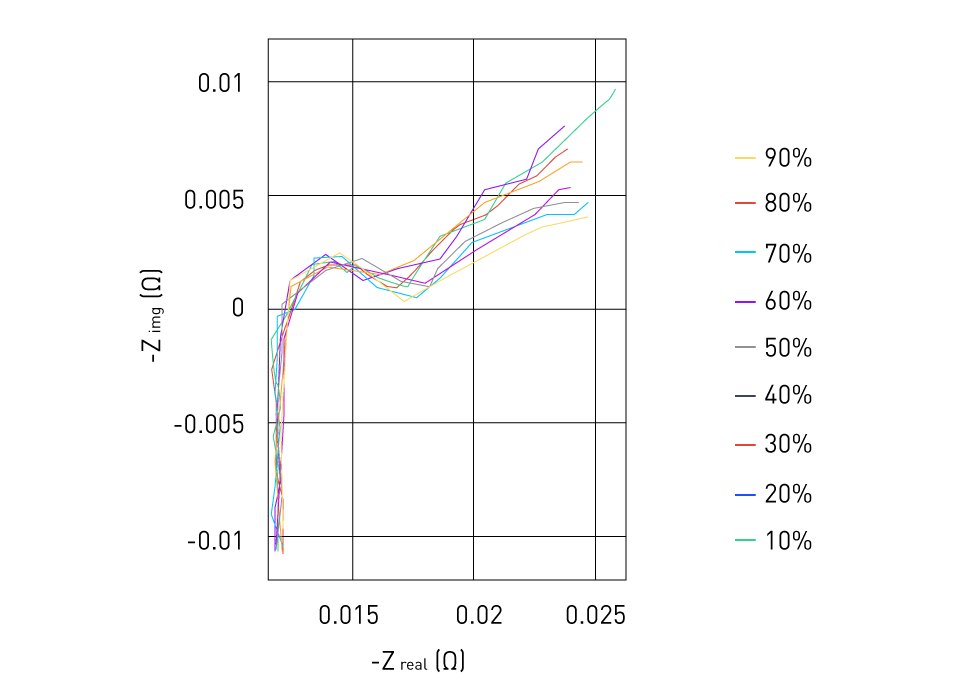
Figure 14: Nyquist plot of a battery discharge
Time-Domain Methods: These techniques entail examining the system's time-domain response to particular excitation signals such as steps in the load current. One can adjust the parameters to get the best fit by comparing the measured and model-generated time-domain responses. The time-domain analysis test method used with a current pulse-stream test is shown in the following plot:
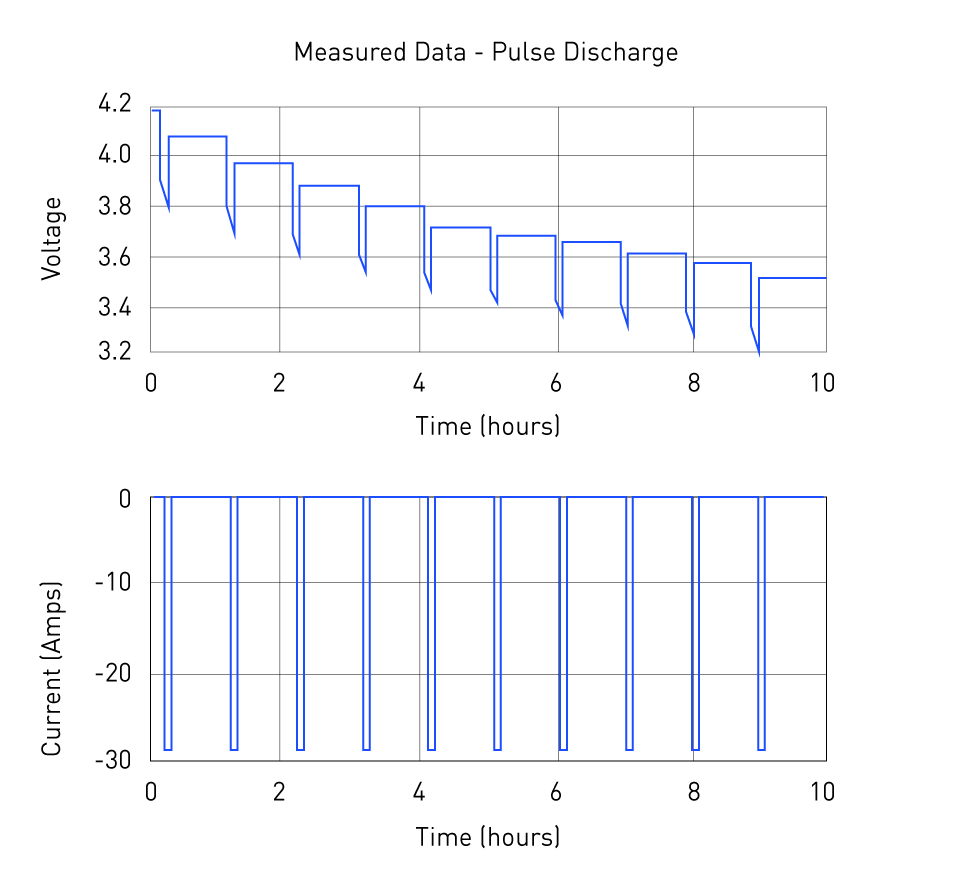
Figure 15: Pulse-stream test of battery
Black-Box Modeling: In some cases, the ECM's structure is unknown beforehand. In these circumstances, system identification can be accomplished using black-box modeling techniques like neural networks. Without necessarily comprehending the inherent dynamics, this method focuses on precisely reproducing the input-output behavior.
Validation of Estimated Parameters
After the parameters of a model have been estimated, it becomes paramount to validate these parameters to ensure that the model faithfully mirrors the real system. The validation process entails evaluating the model's performance through the use of a variety of metrics and techniques.
Goodness of Fit Metrics
This comes into play to quantitatively assess how well the model's predictions align with the actual data. Several goodness of fit metrics are available, and their choice depends on the model's nature and the data.
R-squared (Coefficient of Determination): This serves as a statistical metric that signifies the proportion of the variance in the dependent variable that can be anticipated from the independent variables. Its range spans from 0 to 1, with a value of 1 signifying a perfect fit and 0 indicating no fit whatsoever.
Root Mean Squared Error (RMSE): This is the average of the squared discrepancies between the observed real results and the model's predicted outcomes. It gives an assessment of the prediction error of the model.
Mean Absolute Error (MAE): Without taking into account their direction, MAE calculates the average size of mistakes in a set of forecasts. It is the mean of the absolute differences between forecast and actual observation across the test sample.
Akaike Information Criterion (AIC): When choosing a model, the Akaike Information Criterion (AIC) allows for a trade-off between the model's complexity and goodness of fit.
Cross-validation
A method for determining how well a model's findings will generalize to a different data set is cross-validation. It is primarily used to evaluate a model's performance on a fresh set of data that was not incorporated into the parameter estimation process.
K-Fold Cross-validation: K-fold cross-validation is the variation of cross-validation that is most frequently employed. The data set is split into k subsets using this method. The remaining k-1 subsets are combined to create a training set with one of the k subsets serving as the test set. On the training set, the model is developed, and the test set serves as its validation. Each of the k subsets is utilized as test data exactly once during the k times this process is repeated.
Leave-One-Out Cross-validation: This method constitutes a special instance of k-fold cross-validation, where the value of k equals the number of observations within the dataset. Consequently, each individual observation serves as a test set exactly once.
The application of cross-validation aids in comprehending the model's sensitivity to the data it was trained on, offering insight into how the model is likely to perform when it's employed for making predictions on data that wasn't utilized during the parameter estimation.
The validation of the estimated parameters stands as a pivotal stage in the modeling process. It serves the purpose of evaluating the model's accuracy and resilience, as well as shedding light on its limitations. Both goodness of fit metrics and cross-validation represent potent tools in the validation endeavor.


直接登录
创建新帐号