Time-Domain vs. Frequency-Domain Analysis

Both time-domain and frequency-domain characteristics are present simultaneously in electrical signals and electronic systems. The behavior of electronic circuits and control systems can be understood and predicted using fundamental simulation techniques such as time-domain and frequency-domain analyses. Depending on the nature of the system being evaluated and the unique design goals, each method has distinct benefits. Effective simulation and design in power electronics and control systems depend on an understanding of the differences between these two approaches as well as their corresponding applications.

Figure 6: Time-domain vs. frequency-domain analysis

Time-Domain Analysis

Time-domain analysis examines how different inputs or disturbances affect a system's variables across time, such as voltage, current, or control signals. The system's steady-state and transient behaviors may be directly seen, which makes it very helpful for evaluating dynamic performance.

Applications:

Transient Response: Studying a system's transient response, such as rise time, settling time, overshoot, and oscillations, requires time-domain analysis. When engineers develop a power converter, for example, they utilize time-domain analysis to assess how quickly a control loop reacts to abrupt disturbances or how soon the output voltage stabilizes following a load change.

Switching Behavior in Power Electronics: Time-domain analysis aids in the visualization of switching waveforms and the assessment of switching losses, conduction losses, and electromagnetic interference (EMI) generated by rapid switching events in systems where switching behavior is crucial, such as DC/DC converters or inverters.

Control System Stability: The stability of control systems can also be evaluated using time-domain analysis, specifically by examing how the system reacts to disturbances or setpoint variations over time. This involves determining if there are too many oscillations or instability before the system reaches a steady state.

Tools and Techniques:

SPICE Simulations: For time-domain analysis, circuit simulators such as SPICE are frequently utilized. These tools provide detailed waveforms of voltages and currents at various circuit nodes, simulating the behavior of the circuit over time.

MATLAB/Simulink: The time-domain response of control systems is often modeled and simulated using MATLAB/Simulink. Engineers can use it to build detailed models of controllers, power electronics, and other components and see how the system responds to inputs that change over time.

Advantages:

Direct Observation of Dynamic Behavior: Designing and fine-tuning control systems requires a clear and intuitive knowledge of a system's dynamic behavior, which time-domain analysis offers.

Identification of Transient Issues: This method is highly effective for identifying and fixing transient problems that steady-state analysis could miss, such as overshoot, ringing, and stability issues.

Frequency-Domain Analysis

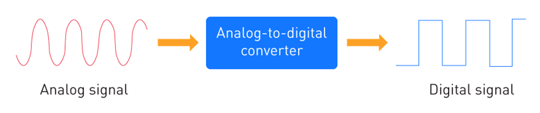
Each signal includes multiple frequency components, and frequency-domain analysis focuses on how a system responds to different signals, each with a unique frequency composition. In the analysis, time-domain signals are represented in terms of their frequency components, and the time domain is transformed to the frequency domain using Fourier or Laplace transforms.

Figure 7: Signal translation between time and frequency domains

Applications:

Bode Plot Analysis: Frequency-domain analysis is frequently used to create Bode plots, which graphically represent a system's phase shift and gain over a range of frequencies. Bode plots are crucial for the analysis and design of feedback control systems because they offer details about the bandwidth, resonance frequencies, and stability margins of the system.

Figure 8: Bode plot

Harmonic Analysis: In power electronics, frequency-domain analysis is also used to study harmonic distortion, especially in systems with nonlinear components such as transistors and diodes. This method allows engineers to design filters that reduce undesirable frequency components and evaluate how harmonics affect system performance.

Impedance and Resonance: Frequency-domain analysis helps in the comprehension of impedance characteristics and the detection of potential resonance issues in power systems and radio frequency (RF) circuits. This is especially useful for designing RF amplifiers, power distribution systems, and matching networks.

Tools and Techniques:

Fast Fourier Transform (FFT): FFT is a mathematical algorithm that converts time-domain signals to their frequency components. It is extensively used in spectral analysis tools such as MATLAB and Simulink to help engineers discover dominant frequencies and harmonics in signals.

Nyquist and Nichols Charts: When designing control systems, these graphical tools help in evaluating stability and visualizing a system's frequency response. Nyquist plots, which show how the frequency response encircles crucial points in the complex plane, are particularly helpful for assessing the stability of closed-loop systems.

Advantages:

Insight into System Stability: Frequency-domain analysis provides a more in-depth understanding of a system's stability and performance under a variety of operating conditions. It is especially useful for designing strong control systems that remain stable even when system dynamics change.

Analysis of Resonance and Filtering: This analysis method is crucial for detecting and resolving resonance issues as well as for designing filters that efficiently eliminate undesired frequency components, enhancing system performance as a whole.

Choosing Between Time-Domain and Frequency-Domain Analysis

Table 5: Comparison between time-domain and frequency-domain analyses

Aspect	Time Domain Analysis	Frequency Domain Analysis
Description	Analyzes how the system's variables change over time, focusing on transient and steady-state behavior	Analyzes the system's response in terms of frequency components, often focusing on steady-state sinusoidal behavior
Primary Focus	Temporal variations of current, voltage, and power over time	The system's response to different frequencies, especially the steady-state sinusoidal behavior
Signal Representation	Signals are represented as time-varying waveforms (e.g., voltage, current)	Signals are represented in terms of their frequency content (using Fourier transforms or Laplace transforms)
Mathematical Tools	Ordinary Differential Equations (ODEs), State-Space models, and simulations	Fourier Transform, Laplace Transform, Bode plots, and Transfer Functions
Key Features	Focus on time-varying signals; Can analyze transients and step responses	Focus on frequency content of signals; Helps in analyzing steady-state sinusoidal responses
Complexity	Can be more complex for systems with non-linear behavior or switching events	More straightforward for linear, time-invariant systems, but can require approximations for non-linear systems
Typical Use Cases	Simulation of switching converters (e.g., buck, boost); Analysis of transient response in filters, feedback systems	Steady-state analysis of filters, impedance, and resonance; Power spectral analysis, harmonic analysis in AC systems
Limitations	Difficult to handle complex or non-linear systems analytically; Can be computationally intensive for transient analysis.	Assumes steady-state conditions, not ideal for transient behavior; Less effective for systems with significant time-varying or non-linear behavior
Advantages	Provides a real-time view of system performance; Can simulate realistic transient events and non-linearities	Simplifies the analysis of steady-state performance; Can easily identify resonance, filtering, and harmonic behavior

Complementary Approaches:

Use in Tandem: In practice, time-domain and frequency-domain analyses are frequently used together because they provide complementary insights into system behavior. Time-domain analysis, for example, can identify transient issues that are subsequently investigated further using frequency-domain techniques to identify their underlying causes and develop appropriate solutions.

System Type and Design Goals: The decision between frequency-domain and time-domain analysis frequently comes down to the principal design objectives and the particular system being designed. When transient performance is crucial for a system, time-domain analysis could be more important. In contrast, frequency-domain analysis is more frequently emphasized for systems where filtering and stability are essential.

Case Study Example:

Power Converter Design: In the design of a DC/DC converter, time-domain analysis is performed to observe the converter's response to a load step, ensuring that transient performance requirements are met. Following that, frequency-domain analysis may be used to evaluate the converter's control loop stability, ensuring sufficient phase and gain margins to prevent oscillations under changing operating conditions.

Non-linear and Linear Simulations

Simulations are essential for predicting system behavior and performance optimization in the analysis and design of power electronics and control systems. Depending on the characteristics of the system under study, these simulations can be broadly divided into linear and non-linear types, each serving different purposes. Understanding the difference between linear and nonlinear simulations, as well as their applications, is critical for accurately modeling and analyzing real-world systems.

Linear Simulations

Linear simulations concentrate on systems that follow the concepts of superposition and homogeneity, in which

• The total of the responses to each individual input is the response to a sum of inputs
• If the input is scaled by a constant, then the output is scaled by the same constant

The relationship between inputs and outputs in linear systems is defined by linear equations, which usually have constant coefficients.

Applications:

Control Systems Analysis: In control systems, linear simulations are widely used, especially during the initial phases of design. Many control techniques, including conventional Proportional-Integral-Derivative (PID) control, are predicated on linear models, which assume that the system functions with minor deviations around a predetermined operating point.

Frequency Response Analysis: Frequency response analysis is simple and offers insightful information on the behavior of linear systems. The performance and stability of control systems are assessed using methods such as Nyquist plots and Bode plot analysis.

Small-Signal Analysis in Power Electronics: Linear simulations are frequently employed in power electronics for small-signal analysis, which linearizes the system around a specific operating point. When designing and adjusting feedback loops in converters, inverters, and other power electronic circuits, this approach is especially useful.

Advantages:

Simplicity and Efficiency: Compared to non-linear simulations, linear simulations require less computing power, which makes them faster and simpler to perform. Early in the design process, when rapid iterations are required to investigate various control strategies or system configurations, this efficiency is especially advantageous.

Predictability and Analytical Solutions: Linear systems can typically be solved analytically, providing transparent and predictable results. Because of this predictability, linear simulations are an effective tool for comprehending how systems behave fundamentally and for developing initial control strategies.

Limitations:

Limited Range of Validity: Linear simulations are only accurate for systems that operate within a limited range around a specified operating point. They fail to account for nonlinearities caused by large signal changes, saturation effects, or other nonlinear behaviors that occur in real-world systems.

Inability to Model Complex Phenomena: Linear simulations are unable to capture phenomena that are prevalent in power electronics and complicated control systems, such as harmonic distortion, bifurcations, and chaos. These demand for a more advanced non-linear strategy.

Table 6: Linear vs. non-linear simulations

Aspect	Linear Simulation	Non-Linear Simulation
Definition	Involves systems where the output is directly proportional to the input, satisfying the principles of superposition and scaling	Involves systems where the output is not directly proportional to the input, often exhibiting complex behaviors like saturation, hysteresis, or chaos
System Behavior	Predictable, proportional relationships between input and output	Complex and may include multiple possible behaviors (e.g., bifurcations, chaos)
Solution Method	Can often be solved using analytical methods (e.g., transfer functions, Laplace transforms) or simple numerical methods	Typically requires numerical methods like finite difference, Newton-Raphson, or custom iterative solvers
Predictability	Highly predictable, with results scaling proportionally to input changes	Less predictable, often sensitive to initial conditions and small changes in input
Modeling Complexity	Simpler to model, as it involves linear equations and systems	More complex to model, as it requires detailed descriptions of system behaviors (e.g., non-linear functions, friction, or material properties)
Examples	- Electrical circuits with resistors, inductors, and capacitors	- Electrical circuits with diodes, transistors, or non-linear resistors
Simulation Tools	Standard tools like SPICE, MATLAB (using linear solvers), Simulink (with linear blocks)	Requires specialized solvers and methods like finite element analysis (FEA), computational fluid dynamics (CFD), or non-linear solvers in MATLAB/Simulink
Time Response	The system response is often easy to compute and analyze, including steady-state and transient responses	The system's time response can be more complex, possibly including oscillations, saturation, and unstable behaviors
Computation Load	Relatively low, as linear systems can be solved with simpler and more efficient algorithms	High computation load due to the complexity of solving non-linear equations and often requiring more time for convergence
Stability	Stability is easier to determine (e.g., using eigenvalue analysis)	Stability is often harder to analyze and may require specialized tools (e.g., Lyapunov methods)
Dynamic Behavior	Often exhibits simple, linear relationships like exponential decay, steady oscillations, or linear growth	May exhibit complex dynamic behavior like bifurcations, chaos, and limit cycles
Real-World Applicability	Suitable for systems operating under small signal conditions or where linear approximations hold	Used for systems where large variations in input or state occur, or where non-linear phenomena dominate (e.g., power electronics, material stress)

Non-linear Simulations

Non-linear simulations are concerned with systems in which the relationship between input and output is non-linear, i.e. the outcome is not directly proportional to its input. Non-linear systems are governed by non-linear differential equations and can exhibit very complicated behavior, including saturation, dead zones, bifurcations, hysteresis.

Applications:

Power Electronics: Switching actions, magnetic saturation, and other factors cause non-linear behavior in many power electronic systems, including motor drives, inverters, and switching converters. Non-linear simulations are required to effectively estimate the behavior of these systems, particularly in large-signal conditions or during transient events.

Control Systems with Non-linear Elements: When a control system has non-linear components, including dead zones, hard limits, or non-linear actuators, non-linear simulations are employed. These simulations help in the development of control strategies that can manage non-linear behavior while maintaining performance and stability.

Stability and Bifurcation Analysis: Nonlinear simulations are essential for researching the stability of systems that may exhibit bifurcations, in which a tiny change in input or parameters can result in a substantial shift in system behavior. This kind of study is crucial for comprehending the conditions that could cause a system to operate in an unstable manner.

Techniques:

Time-Domain Non-linear Simulation: Time-domain non-linear simulations examine the system's behavior throughout time, considering all nonlinearities. This method is frequently used to solve the system's non-linear differential equations in combination with numerical methods such as Runge-Kutta.

State-Space Modeling: State-space modeling, in which a system is described by a system of non-linear differential equations, is another method for modeling non-linear systems. Systems with multiple interacting variables or those with distributed non-linearities benefit greatly from state-space modeling.

Piecewise Linear Approximation: In some cases, non-linear systems can be approximated by breaking them into many linear segments, each representing a different operational area. While this approach simplifies the analysis, it retains the system's basic nonlinear characteristics.

Advantages:

Comprehensive Modeling: Real-world systems can be more accurately and thoroughly modeled by non-linear simulations, which consider all the complexities and non-linearities that linear models are unable to represent.

Ability to Model Complex Phenomena: Complex phenomena including chaos, harmonic generation, and bifurcations can be captured by non-linear simulations, which is essential for comprehending the complete behavior of power electronics and advanced control systems.

Challenges:

Computational Intensity: Nonlinear simulations are more computationally intensive than linear simulations. They frequently demand more time and resources to run, especially for highly complex systems or when precise precision is required.

Sensitivity to Initial Conditions: Due to their high sensitivity to initial conditions, non-linear systems can produce widely different results from slight variations in input or system parameters. This sensitivity can complicate the design and analysis process, necessitating a thorough evaluation of all potential operational scenarios.

Choosing Between Linear and Non-linear Simulations

System Characteristics:

Dominantly Linear Systems: Linear simulations are usually sufficient and offer quick, reliable insights for systems that behave predominantly in a linear way over the expected operating range. These are often utilized in early-stage design and for systems with few or well-controlled nonlinearities.

Strongly Non-linear Systems: Non-linear simulations are necessary to accurately predict the performance of systems that display considerable non-linear behavior, such as switching power supplies, non-linear control systems, or systems with components operating in different regimes (e.g., saturation, cut-off).

Design Phase Considerations:

Early Design Stages: Linear simulations are frequently used in the early stages of design to quickly explore the design space and develop a baseline understanding of system behavior. As the design evolves and more detailed information is required, non-linear simulations become crucial for refining the design and ensuring robustness under all operating conditions.

Verification and Validation: Non-linear simulations are essential in the verification and validation phases where the system must be tested in a range of scenarios to make sure it performs as planned in real-world conditions.

Complementary Use:

Iterative Approach: In real-world applications, engineers frequently employ an iterative combination of linear and non-linear simulations. Non-linear simulations improve the design by capturing detailed behavior and resolving potential issues that linear models might overlook, whereas linear simulations are used to develop initial designs and obtain broad understanding.

Parametric Sweeps and Sensitivity Analysis

In simulation, parametric sweeps and sensitivity analysis are essential techniques for investigating how changes in system parameters impact overall performance. These methods allow engineers to systematically explore the effect of essential variables, such as component values or control parameters, on the behavior of electronic circuits, power systems, or control systems.Engineers can improve robustness, optimize designs, and ensure the system operates reliably under a variety of operating conditions by comprehending the connections between various parameters and system performance.

Parametric Sweeps

The process of parametric sweeping involves methodically changing one or more simulation model parameters to observe how these changes impact system behavior. The parameters could include operating voltages, control gains, environmental conditions, or component values (such as resistor or capacitor values).

Applications:

Circuit Optimization: Parametric sweeps are often used to study and enhance electrical circuits by adjusting component values (e.g., resistance, capacitance, inductance) to achieve desired performance, such as improved frequency response, reduced power losses, or increased stability.

Control Systems Tuning: Parametric sweeps are used in control systems to explore how the stability and transient response of the system are affected by changing control gains (such as proportional, integral, and derivative gains in a PID controller). Engineers can determine the ideal set of parameters that yield the optimum control performance by sweeping through a range of values.

Power Electronics Design: The efficiency, power factor, and overall operation of converters, inverters, or motor drives can be examined using parametric sweeps in power electronics to examine the effects of changes in switching frequency, duty cycle, or input/output voltages.

Execution:

Single-Parameter Sweeps: A parametric sweep is most simply defined as changing a single parameter over a specific range while keeping all other parameters constant. This enables the engineer to focus on the precise effects of a single variable on system performance.

Figure 9: Single-parameter (frequency) sweep for a low-pass filter

Multi-Parameter Sweeps: In more complex sweeps, multiple parameters are changed simultaneously. Because there are more simulations involved, these multi-dimensional sweeps offer a more thorough understanding of the interactions between parameters, but they also come with higher processing requirements.

Table 7: Single- vs. multi-parameter sweeps

Aspect	Single Parameter Sweep	Multi-Parameter Sweep
Number of Parameters	Involves varying one parameter at a time	Involves varying multiple parameters simultaneously
Complexity	Simpler to set up and analyze	More complex due to interactions between parameters
Results Analysis	Easier to interpret, as only one parameter is changing	More complex analysis due to the combination of multiple variables
Use Case	Suitable for understanding the effect of a single variable	Useful for exploring how multiple factors interact
Computational Load	Generally lower, as only one parameter is varied	Higher computational load, as multiple simulations are needed
Time Efficiency	Faster, as fewer simulations are required	Slower, due to the larger number of simulations needed

Benefits:

Optimization and Fine-Tuning: Parametric sweeps enable the systematic optimization of system parameters, ensuring that the design matches performance requirements while reducing trade-offs including heat dissipation or power consumption.

Comprehensive Exploration of Design Space: Parametric sweeps assist guarantee that the design is robust and functions effectively under a variety of operating conditions by exploring with a wide range of parameter values. This is especially crucial for designs that must function in dynamic environments or with a variety of inputs.

Sensitivity Analysis

Sensitivity Analysis determines how sensitive a system's output is to variations in its input parameters. It helps engineers prioritize specific design variables over others by determining which parameters have largest effects on system behavior.

The sensitivity of an output f to an input parameter x_i is mathematically described as the partial derivative with respect to x_i:

$$ S_{x_i} = \frac{\text{Percent change in output}}{\text{Percent change in input}} = \frac{\partial f(x_1, x_2, x_3, \ldots, x_n)}{\partial x_i} $$

This calculates the rate of change in the output f when the parameter x_i is changed while all other inputs remain constant.

Applications:

Robust Design: Designing robust systems that can withstand changes in manufacturing, environmental conditions, or operational fluctuations requires sensitivity analysis. By identifying the most important parameters, engineers can focus on strictly controlling these variables during the manufacturing process or develop compensatory strategies to lessen their effects.

Failure Analysis: Sensitivity analysis is frequently employed in failure analysis to determine the underlying cause of faults in systems. Engineers can identify the most likely causes of failure or performance degradation by simulating small parameter changes and tracking their effects.

Tolerance Analysis: Sensitivity analysis aids in determining how changes within tolerances impact overall performance in circuits or systems that involve components with tolerances (such as resistors, capacitors, and inductors). This enables engineers to ensure reliable operation by specifying appropriate tolerance levels for components.

Execution:

Direct Sensitivity Analysis: Direct sensitivity analysis involves varying each parameter slightly and measuring the resulting change in system output. The ratio of the output change to the input parameter change is then used to determine the sensitivity. This provides a quantifiable measurement of how much each parameter affects system performance.

Global Sensitivity Analysis: Global sensitivity analysis involves changing all parameters across the full range simultaneously and assessing the combined effect on system behavior. Although this approach offers a more thorough understanding of the system's sensitivity, it needs more complex simulations and more computational resources.

Sensitivity Coefficients: Sensitivity coefficients can be calculated to offer a normalized measure of how each parameter impacts the system. These coefficients are useful for assessing the relative relevance of different parameters, especially when their units or magnitudes differ.

Benefits:

Identifying Critical Parameters: Sensitivity analysis aids in determining which parameters most significantly affect system performance. While less significant parameters can be given lower priority or wider tolerances, this enables engineers to concentrate on enhancing these crucial parameters.

Improving Robustness: Engineers can design systems that are less vulnerable to variations in performance by understanding which parameters are most sensitive. As a result, designs become more resilient to variations in component tolerances or operating conditions that occur in the real world.

Differences Between Parametric Sweeps and Sensitivity Analysis

Parametric Sweeps:

• Examine how variations in one or more parameters impact system performance over a broad range of values.
• Usually employed in optimization, where identifying the optimum combination of parameter values for peak performance is the aim.
• Engineers can see the system's behavior over a wide range of design spaces thanks to its focus on design exploration.

Sensitivity Analysis:

• Focuses on measuring the system's sensitivity to even little changes in input parameters.
• Used to determine which parameters have the most effects on system performance and behavior.
• It emphasizes which parameters require strict control to maintain reliable performance, making it more focused on robustness and failure prevention.

Combining Parametric Sweeps and Sensitivity Analysis

Iterative Approach:

In practice, parametric sweeps and sensitivity analysis are frequently used together. Engineers may begin with parametric sweeps to explore the whole design space and optimize the system, then utilize sensitivity analysis to identify important factors that require tighter control during production or operation.

This iterative process guarantees that the system is both highly efficient and resilient to changes while enabling thorough optimization.

Monte Carlo Simulations and Worst-Case Scenario Analysis

The robustness, reliability, and performance of systems under various conditions and uncertainties are evaluated by engineers using Monte Carlo simulations and worst-case scenario analysis, which are crucial methods in engineering design and analysis, especially in domains such as power electronics, control systems, and circuit design. These methods enable thorough evaluation and guarantee that designs satisfy performance and reliability standards by accounting unpredictability, variability, and extreme cases.

Monte Carlo Simulations

Monte Carlo simulations model the impact of random changes in system parameters on overall performance using statistical techniques. These simulations, which are named after the well-known casino in Monaco, use repeated random sampling to predict how input variable uncertainties impact system behavior.

Applications:

Component Tolerance Analysis: Monte Carlo simulations are frequently used to examine the effects of changes in component tolerances (such as those of resistors, capacitors, and inductors) on electronic circuit performance. Small changes in component values, for example, may have an impact on a power converter's output voltage, efficiency, and thermal performance. Monte Carlo simulations aid in determining the probability that these variations will result in a decline in performance.

Statistical Reliability Evaluation: Monte Carlo methods are used in reliability engineering to predict the probability of system failure or performance decline as a result of aging components, environmental impacts, or random manufacturing variances. This is especially helpful in crucial industries where reliability is crucial, such as medical electronics, automotive, and aerospace.

Stochastic Control Systems: Monte Carlo simulations in control systems can help determine how random fluctuations in sensor readings, actuator responses, or environmental conditions affect control performance. Engineers can predict the distribution of results and assess the probability of undesired behavior, including instability or excessive overshoot, by modeling the system's response to a large number of random inputs.

Table 8: Monte Carlo Simulation

Aspect	Explanation
Definition	A computational method that uses random sampling to obtain numerical results for systems with uncertainty or complex models
Purpose	To model the probability of different outcomes in a process that cannot easily be predicted due to presence of random variables
Key Components	Random inputs or variables (e.g., probability distributions) Repeated simulations to generate a distribution of outcomes
Process	Define a probabilistic model of the system Randomly sample values based on defined distributions Perform simulations using these input values Analyze the output to estimate probabilities, mean, variance, etc
Types of Problems Solved	Optimization Predicting outcomes with uncertainties
Output	A range of possible outcomes and their probabilities, often visualized as histograms, probability distributions (PDFs), or cumulative distribution functions (CDFs)
Key Advantage	Handles complex problems with multiple uncertain variables where analytical solutions may not be feasible
Key Disadvantage	Computationally intensive, especially with large numbers of simulations or complex models
Assumptions	Assumes that the inputs are random and follow defined probability distributions
Output Analysis Techniques	Statistical techniques like mean, standard deviation, confidence intervals, histograms, and cumulative distribution curves

How It Works:

Random Sampling: Monte Carlo simulations treat system parameters as random variables, with each parameter having a specified probability distribution (normal, uniform, or exponential). A huge number of random samples are taken from these distributions, and the system is simulated for each set of random inputs.

Figure 10: Probability distribution functions

Statistical Analysis of Results: A distribution of system outputs is obtained by statistically analyzing the simulation's results after thousands or even millions of iterations. The probability that the system will fulfill its performance requirements or fail because of unfavorable parameter combinations is one of the outcomes that engineers can then evaluate.

Benefits:

Robustness Evaluation: Monte Carlo simulations are an effective method for determining the resilience of a design by accounting for all conceivable variations in input parameters. This approach guarantees that the system will function consistently in real-world conditions, where ideal operating conditions or component values cannot be presumed.

Probabilistic Design: Monte Carlo simulations allow engineers to design for a variety of potential outcomes rather than focusing on a single "nominal" design point. This aids in developing systems that are reliable under ambiguous conditions and less susceptible to fluctuations.

Worst-Case Scenario Analysis

Worst-case scenario analysis examines a system's performance in the worst-case scenarios, usually considering the worst possible combination of input parameter values. This approach guarantees that the design can survive the most challenging conditions it may face in practice and identifies the absolute limits of system performance.

Applications:

Safety-Critical Systems: Worst-case scenario analysis is critical in applications such as aerospace, medical devices, and automobile safety systems to ensure that the system remains operational and safe even under the most extreme or unforeseen scenarios. For example, in a medical device, engineers must verify that the system continues to function properly even when environmental conditions such as temperature or humidity reach high levels.

Power Electronics Stress Testing: Worst-case analysis is used in power electronics to assess the effects of extreme operating conditions on performance, such as maximum load, minimum supply voltage, or worst-case thermal conditions. This guarantees that components such as capacitors, diodes, and transistors won't malfunction under extreme conditions.

Control Systems Stability: Worst-case scenario analysis is used in control system design to evaluate whether the system is stable and responsive in the worst-case scenarios, such as severe sensor noise, abrupt changes in maximum load, or delayed feedback signals.

How It Works:

Identification of Critical Parameters: The first stage in worst-case scenario analysis is identifying the essential parameters that, if exceeded, could cause system failure or inadequate performance. Component tolerances, operating conditions (voltage, current, load), and environmental factors (temperature, humidity) are a few examples of these parameters.

Simulating Extreme Conditions: The system is simulated using the most extreme values of the crucial parameters after they have been identified. The worst-case scenarios of a power converter, for instance, could include the maximum working temperature, minimum input voltage, and maximum load. To make sure the system maintains performance and safety standards, engineers assess how it functions in these extreme conditions.

Safety Margins and Redesign: In order to improve robustness, engineers might need to include safety margins or modify some components if the system doesn't function well in the worst-case scenario. This could entail introducing redundancy, employing higher-rated components, or modifying the control system to deal with the worst-case scenarios.

Benefits:

Ensures Reliability in Extreme Conditions: Worst-case scenario analysis ensures that the system will perform properly even under the most challenging conditions it may face over its lifetime.

Prevents Catastrophic Failures: Worst-case scenario analysis helps prevent catastrophic failures by identifying potential failure points prior to system deployment, especially in safety-critical systems where failure could result in loss of life or considerable financial loss.

Differences Between Monte Carlo Simulations and Worst-Case Scenario Analysis

Monte Carlo Simulations:

Focus on Probabilities: Monte Carlo simulations use random parameter changes to investigate the full range of potential outcomes. The purpose is to calculate the probability distribution of outcomes and assess the risk of failure or performance degradation.

Statistical Insight: These simulations assist engineers design for resilience and reliability across a range of inputs by offering statistical insights into how a system behaves under different conditions.

Comprehensive Analysis: Monte Carlo simulations are more comprehensive since they consider a wide range of parameter values rather than just the extremes.

Worst-Case Scenario Analysis:

Focus on Extremes: Worst-case scenario analysis focuses on the most extreme operating situations and examines how the system works under it.

Safety and Margins: To make sure the system has enough safety margins and can withstand the worst-case scenarios; this study is frequently employed in safety-critical applications.

Deterministic: Worst-case scenario analysis is deterministic, concentrating on the single worst-case set of parameters rather than a distribution of potential values, in contrast to Monte Carlo simulations, which are probabilistic in nature.

Complementary Use of Monte Carlo Simulations and Worst-Case Scenario Analysis

Worst-case scenario analysis and Monte Carlo simulations are frequently combined in engineering applications to offer an extensive understanding of system performance. Monte Carlo simulations are useful for assessing probabilistic results and ensuring the system functions well when parameters vary in normal conditions. On the other hand, worst-case scenario analysis finds potential areas of failure in the worst-case scenario and guarantees that the system can endure extreme conditions.