Understanding Response Time in Control Systems

In control systems, response time is a crucial parameter that establishes how fast a system responds to input or setpoint changes. It has a direct effect on the system's capacity to sustain the stability and performance that are needed, particularly in dynamic conditions. The notion of response time, the factors influencing it, and its importance in analog and digital control systems are explored in this section.

Definition of Response Time

In control systems, response time is the amount of time it takes for the system to react to a change in input and reach at a new setpoint or equilibrium. It is crucial to realize that the response time of the system is dependent upon the response times of each component of the control system. When compared to the response times of other components of the control system, the controller's (analog or digital) response time can be negligible.

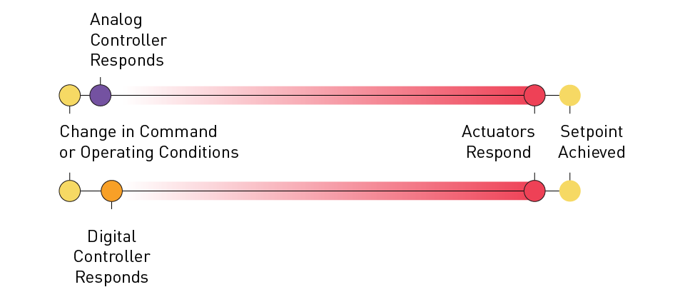
Figure 1: Digital vs. Analog Controller Response Times

There are multiple components that make up the system response time:

Delay Time: The amount of time needed to get to 50% of the final value.

Rise Time: The amount of time needed for the system output to increase from a low value (typically 10% of the final value) to a high value (typically 90% of the final value).

Peak Time: The amount of time needed to get to the highest overshoot (or peak) value.

Settling Time: The time required for the system output to remain within a specific percentage (e.g., 2% or 5%) of the final value following an input change.

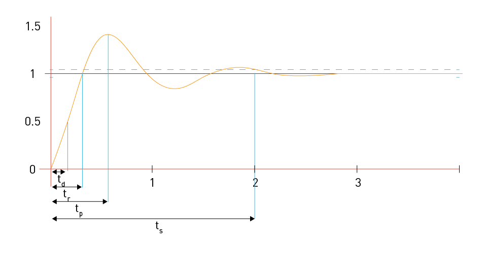
Figure 2: Response time components

Factors Affecting Response Time

System Dynamics:

Natural Frequency: The system has an inherent oscillatory behavior. Systems with higher natural frequencies typically have faster response times.

Damping Ratio: A measure of how a system's oscillations decrease following a disruption. Overdamped systems respond slower, whereas underdamped systems may oscillate before settling.

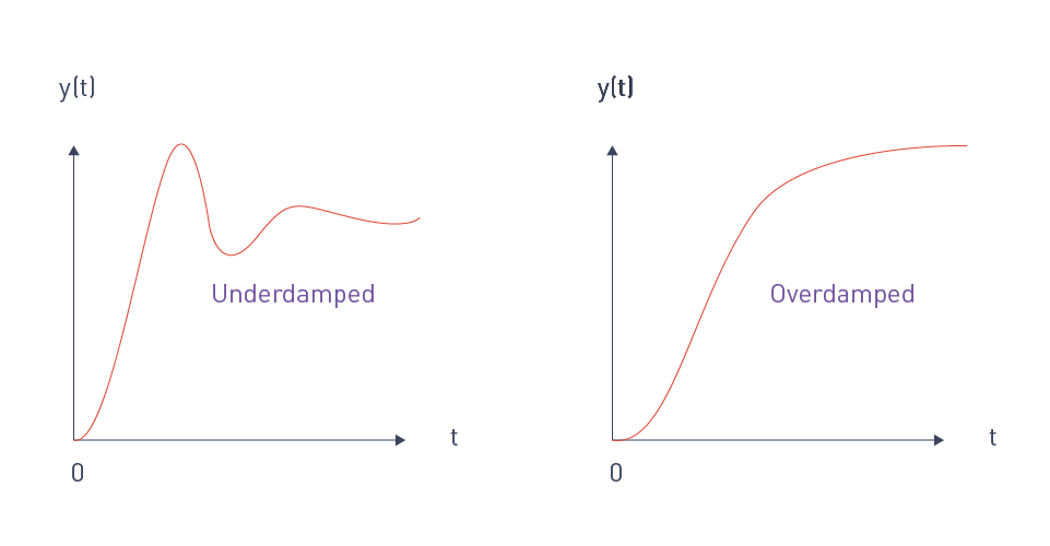
Figure 3: Underdamped vs. overdamped systems

Control Algorithm:

PID Parameters: Response time in a PID controller is greatly impacted by the proportional, integral, and derivative gains. Although they may increase oscillations and overshoot, higher proportional gains can decrease response time.

Sampling Rate: Response time in digital systems is influenced by the frequency at which the controller samples the input signal. Although they demand more processing power, higher sample rates can improve response times.

System Inertia:

Mechanical Systems: Physical mass and friction have an effect on response speed in systems with a lot of inertia, including motors and mechanical linkages.

Electrical Systems: Response time is impacted by the delays introduced by inductance and capacitance in electrical systems.

Feedback Loop:

Feedback Gain: The strength of the feedback signal influences how quickly the system corrects deviations from the setpoint.

Sensor and Actuator Dynamics: The overall response time of the system is also influenced by the response times of the sensors and actuators. Slow sensors or actuators may restrict how fast the system responds.

Response Time in Analog vs. Digital Control Systems

Analog Control Systems:

Continuous Processing: Continuous signal processing in analog systems enables almost immediate responses to input changes.

Speed of Components: The response time is determined by the speed of analog components like capacitors and op-amps. High-speed response times are possible with high-speed analog components.

Digital Control Systems:

Discrete Processing: The sampling rate and processing speed determine the response time of digital systems, which sample inputs at discrete intervals.

Algorithm Execution: The overall response time is impacted by the amount of time needed to run control algorithms on a microcontroller or DSP.

Significance of Response Time

Performance:

Quick Response: crucial for applications that need fast adjustments, like automotive systems, robotic arms, and aerospace controls.

Slower Response: Acceptable in systems such as industrial process controls and climate control systems where precision and stability in the steady state are more important than speed.

Stability:

Fast Response: If not adequately damped, systems with extremely fast response times run the risk of becoming unstable and experiencing oscillations and overshoot.

Optimized Response: It is essential to strike a balance between stability and speed. Reducing response time by overly aggressive tuning can compromise stability.

Accuracy:

Transient Accuracy: Fast response times improve the system's capacity to accurately track changes with minimal delay.

Steady-State Accuracy: The system must settle precisely at its ideal setpoint, with no lengthy oscillations or drift.

Energy Efficiency:

Power Consumption: Faster response times can lead to more power consumption, especially in digital systems with high processing requirements and sampling rates.

Thermal Management: Power electronics' rapid responses can produce heat, thus efficient thermal management strategies are required.

Analyzing Accuracy: Error Sources and Mitigation in Analog and Digital Systems

A control system's accuracy is a crucial indicator of its capacity to produce and sustain the intended output. It shows how closely the output of the system resembles the reference signal or setpoint. Accuracy can be affected by a variety of error sources in both analog and digital control systems. In order to improve accuracy, this section explores the common causes of errors in these systems and discusses strategies to reduce them.

Error Sources in Control Systems

Sensor Errors:

Analog Control: Errors can be introduced by analog sensors because of noise, drift, and non-linearities.

Digital Control: Resolution limits and quantization errors are other issues that digital sensors encounter.

Component Tolerances:

Analog Control: Inaccuracies may result from variations in component values (capacitors, resistors, etc.).

Digital Control: Despite being less vulnerable to component fluctuations, tolerances in ADCs and DACs can still have an impact on digital systems.

Noise and Interference:

Analog Control: Signal distortion can result from noise and electromagnetic interference, which are more common in analog systems.

Digital Control: Although digital systems are more resistant to noise, high-frequency noise can still affect digital circuits.

Quantization Errors:

Analog Control: Quantization errors are not an issue for analog systems because they process continuous signals.

Digital Control: During the analog-to-digital conversion process, digital systems inherently generate quantization errors.

Algorithmic Errors:

Analog Control: Drift and component tolerances can have an impact on analog control algorithms that are implemented through circuit components.

Digital Control: Software-implemented digital control algorithms can cause errors due to finite word length and numerical precision.

Mitigation Strategies

Calibration and Compensation:

Analog Control: Regular calibration of analog components can help reduce errors caused by component tolerances and drift.

Digital Control: Algorithms for software-based compensation can correct quantization effects and sensor errors.

Filtering and Noise Reduction:

Analog Control: employing low-pass and high-pass analog filters to minimize signal noise and interference.

Digital Control: Noise in sampled signals can be eliminated using digital filtering techniques.

Precision Components:

Analog Control: Accuracy can be improved by using low-tolerance, high-precision components.

Digital Control: Reduce quantization errors by selecting high-resolution ADCs and DACs.

Algorithm Optimization:

Analog Control: Analog circuit design is optimized to reduce the impact of component tolerances and drift, followed by field calibration.

Digital Control: Applying numerical algorithms that improve precision and reduce rounding errors.

Shielding and Grounding:

Analog Control: Proper grounding and shielding techniques to reduce electromagnetic interference.

Digital Control: To protect digital circuits from high-frequency noise, implement grounding and shielding.

Stability Criteria in Control Systems: Bode Plots, Nyquist Criteria, etc.

Stability is a crucial requirement for control systems, since it ensures that the system maintains controlled behavior and does not exhibit unbounded or oscillatory responses over time. Bode plots, Nyquist criteria, and root locus techniques are a few of the mathematical tools and criteria used in stability analysis and verification. This section explores these techniques and offers an understanding of their application in the evaluation and design of stable control systems.

Bode Plots

Bode plots are graphical representations of a system's frequency response, made up of two plots: magnitude (gain) vs frequency and phase versus frequency.

Magnitude Plot: Demonstrates how the amplitude of the output signal changes with frequency.

• Key Features: Plot slope (a steeper slope indicates a faster change in gain with frequency), bandwidth (the range of frequencies where the system effectively passes signals with minimal attenuation), and gain crossover frequency (the frequency at which the magnitude of the system's transfer function crosses the 0 dB line, meaning the gain is 1 or unity).

Phase Plot: Represents the system's phase shift as a function of frequency.

• Key Features: Phase margin is the difference between the phase at the gain crossover frequency and -180 degrees, and phase crossover frequency is the frequency at which the phase shift reaches -180 degrees.

Figure 4: Bode plot

Stability Analysis:

• Gain Margin: The amount of gain increments necessary to make the system unstable. It is the dB difference between the gain at the phase crossover frequency and 0 dB.
• Phase Margin: The extra lag in phase needed to push the system over the edge of instability. It is the degree difference between the phase at the gain crossover frequency and -180 degrees.
• Criterion: If the gain and phase margins are both positive, the system is stable. This is due to the fact that gain and phase margins indicate the distance from unstable points, and larger margins indicate increased stability.

Figure 5: Phase and gain margins

Nyquist Criteria

The Nyquist criterion is a graphical technique that analyzes the open-loop frequency response of a closed-loop control system to determine its stability.

Nyquist Plot: Plots the open-loop transfer function's complex value.

as the frequency varies from -∞ to +∞.

Stability Analysis:

• Encirclement Criterion: The number of clockwise encirclements of the critical point (-1, 0) on the Nyquist plot is crucial for determining Nyquist stability.
• Criterion: The number of clockwise encirclements of the point (-1, 0) must equal the number of poles of the open-loop transfer function in the right-half s-plane for a system to be considered stable.

Root Locus

The root locus is a graphical method used to analyze how changes in a specific parameter, usually the gain K, affect the roots of a system's characteristic equation.

Root Locus Plot: Plots the potential closed-loop pole locations in the s-plane as the gain K changes from 0 to ∞.

Stability Analysis:

• Poles and Zeros: As the gain changes, the plot displays how the transfer function's poles and zeros change.
• Criterion: If every closed-loop pole stays on the left-half s-plane for every value of K, the system is stable.

Routh-Hurwitz Criterion

The Routh-Hurwitz criterion looks at the characteristic equation without explicitly solving for its roots, offering a methodical way to assess a system's stability.

Routh Array: Uses the characteristic polynomial's coefficients to create an array (Routh array).

Stability Analysis:

• Criterion: If every element in the Routh array's first column is positive, the system is stable. Any changes in sign reveal the number of poles in the right half-plane and, consequently, the instability of the system.

Implications of Stability Criteria

Design Implications: The design of controllers is guided by stability criteria, which guarantee that the control system maintains the intended performance without any divergence or oscillations.

Performance Trade-offs: Other performance metrics, including robustness and transient response, are impacted by stability margins.

Practical Considerations: Non-idealities such as component tolerances, environmental variations, and non-linearities must be taken into consideration in real-world systems.

Implications of Response Time, Accuracy, and Stability in System Performance

Stability, accuracy, and response time are crucial attributes that determine control systems' overall performance. The system's ability to achieve the desired outcomes in a variety of applications is severely affected by these interconnected parameters. Understanding their consequences aids in the design of systems that satisfy performance standards and function reliably under a variety of conditions.

Response Time

Response Time: It is the amount of time needed for a system to respond to a change in input and arrive at a new setpoint or equilibrium. Rise time, settling time, delay time, and peak time are important factors.

Speed of Response: In applications like robotics, aerospace, and automotive systems, where fast adjustments are required to maintain performance, fast response times are essential.

Transient Performance: Response times that are shorter enhance the system's capacity to manage brief fluctuations without experiencing significant oscillation or overshoot.

Energy Efficiency: Faster systems can be more energy efficient because they spend less time in transient states, which reduces energy waste.

Accuracy

Accuracy: It is the degree to which the system's output, considering factors like sensor accuracy, component tolerances, and error sources, matches the intended setpoint or reference value.

Performance: In applications that need precise control, such medical devices and precision manufacturing, high accuracy guarantees that the system operates near the desired setpoint.

Quality and Reliability: Reliability and quality of the end product or process are improved by accurate control systems.

Error Mitigation: High-accuracy systems feature safeguards against errors from multiple sources, ensuring consistent performance.

Stability

Stability: It is a control system's capacity to sustain regulated behavior and regain equilibrium following a disturbance. Typically, stability analysis uses techniques like Nyquist criteria and Bode plots to examine how the system responds to perturbations.

System Reliability: For control systems to be reliable and predictable, stability is essential.

Robustness to Disturbances: Systems that are stable can withstand both internal and external disturbances without substantially deviating from the intended performance.

Design and Maintenance: Control system maintenance requirements and design complexity are influenced by stability.

Interrelationships and Trade-offs

Balancing Response Time and Stability:

Trade-off: Sometimes stability is compromised in order to achieve fast response times, which can result in oscillations and overshoot.

Design Consideration: By properly adjusting and improving control parameters, engineers must strike a balance between the need for reliable operation and fast responses.

Balancing Accuracy and Stability:

Trade-off: Stability can be impacted by increasing accuracy through high-gain feedback, especially if the system becomes too susceptible to noise and disturbances.

Design Consideration: High accuracy can be attained without compromising stability by utilizing strategies like filtering and robust control algorithms.

Impact on System Performance:

Overall Performance: A control system's overall performance is determined by the interplay of response time, accuracy, and stability. To satisfy certain application requirements, each parameter must be optimized with respect to the others.